Dice and Queues

Introduction

One of the key insights from queuing theory is that the average queue size for an unbounded system tends to increase significantly as utilization approaches 100%. Theoretical models show no bound to this increase and at 100% utilization the resulting average queue size grows toward infinity. This is important because queues themselves consume resources, be it memory or disk space on a computer or factory floor space in a plant. In an ideal world, we wouldn’t need queues. Who likes waiting in lines after all? This would only be possible if the arrival rate of items in a queue was less than or equal to the departure rate and there were no variability in either. Not likely to happen in the real world.

Queuing models are often expressed using Kendall Notation (e.g. M/M/1 or M/D/1). These models specify different arrival and departure distributions, such as Poisson or Deterministic. They end up having closed-form expressions that define the average queue size as a function of different system parameters. While these equations are fairly easy to use, I wanted to get a more intuitive understanding of how these models behave and decided to build a simulation based on the idea of rolling a single die many times.

Theory and Simulation Setup

A queue is fairly simple to visualize. In the image below we have a queue with 5 items as well as 1 being serviced. This is a first in first out (FIFO) queue, so as an item arrives it must wait on all items ahead of it to be serviced before it can exit the queue. There is also one item inside of the block labeled “server”. This item is not in the queue, but it’s still considered part of the “system”. So in our example here, we have a queue size of 5 with a total of 6 items in the system.

The arrival rate (λ) is the average rate of items entering the queue. The service or departure rate (μ) is the average rate of items leaving the queue. Both of these rates are expressed in terms of items per unit of time (e.g. 10 items/minute). It’s easy enough to reason that if the arrival rate exceeds the departure rate, the queue size will tend to increase with time. Likewise if the arrival rate is lower than the departure rate, the queue size will tend to decrease over time. What is interesting is the way queues behave when, like in many real world systems, there is variability around the average values.

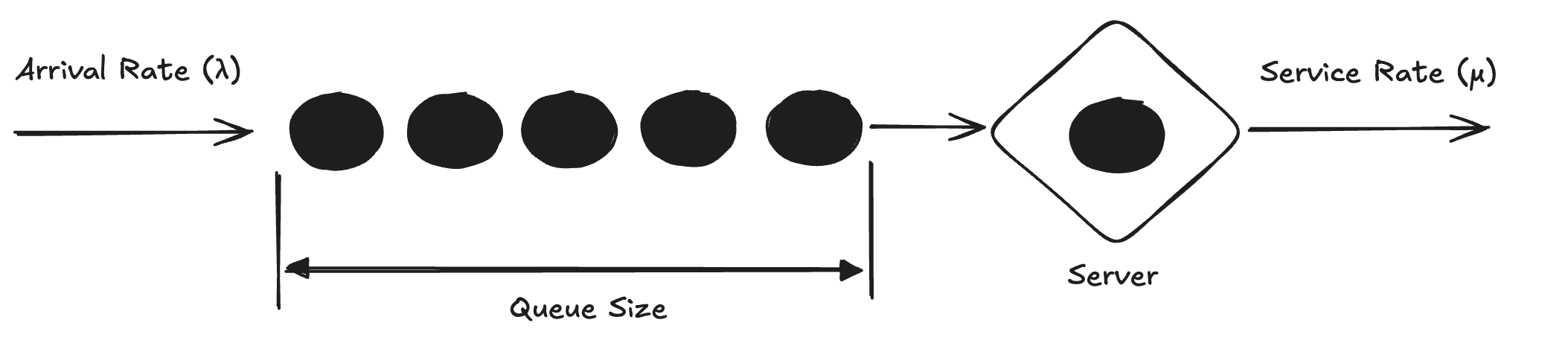
A metric that is useful in analyzing the behavior of queue systems is the utilization factor (ρ). This helps estimate what percentage of time the server is busy.

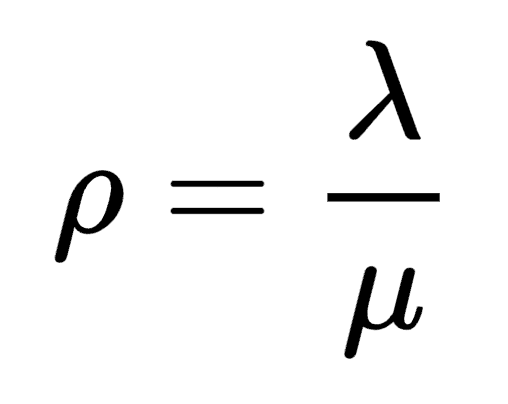
Theory and empirical evidence show that when the utilization factor tends towards 0, so does the average queue size. However, as the utilization factor approaches 1, the queue size can increase significantly. If the utilization factor is greater than 1, it means the average arrival rate is larger than the service rate and the queue will keep growing without stop.

To better understand these dynamics, let’s consider an expiriment where we split up a minute into 60 seconds and at each second we throw a 6 sided die. If the die lands on a 6, we tally a count into our notebook. At the end of the minute, we add up all of our counts. This will be the number of item arrivals we have in our queue in a given minute. The idea here is that all arrivals are equally likely and none of them depend on each other.

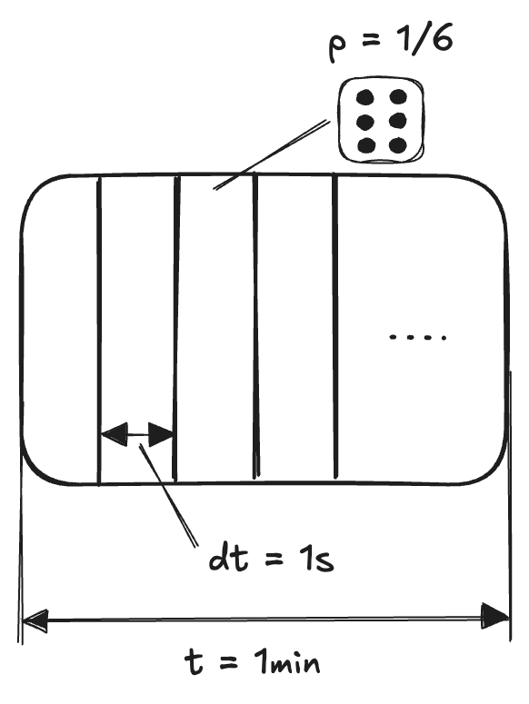
Rather than exhausting our hands throwing a die hundreds of times, we can write a python function, arrivals(), to simulate the scenario described above. Note that each die throw has a 1/6 chance of landing on a 6. We can use the random() function, which returns a uniformly random decimal value between 0 and 1. Each time it returns a value less than 1/6, we increment our count.

def arrivals():
    """
    This function simulates 60 roles of a die and
    returns the number of times a single face
    (e.g. 6) shows up. This simulates a binomial
    distribution where the expected value is
    E[X] = n * p = (1/6) * 60 = 10.
    """
    p = 1 / 6 # chances of rolling a six
    n = 60    # number of rolls
    count = 0
    for i in range(n):
        if random.random() < p: count += 1
    return count

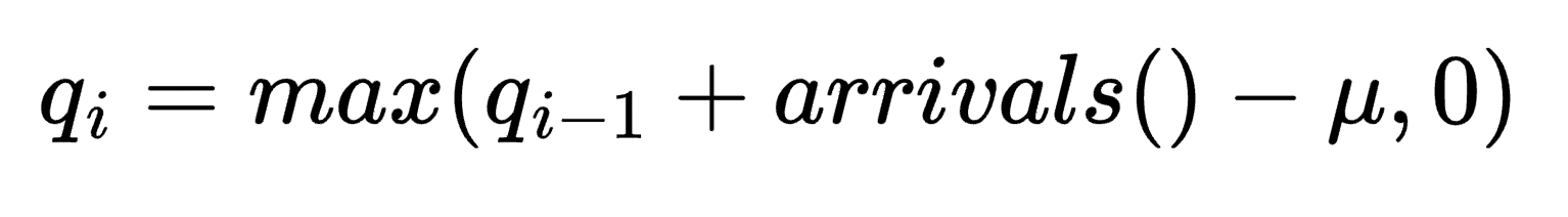
So we now have a mechanism to randomly generate arrivals. For the service rate (λ), we can keep things simple and assume that our server can service 10 items per minute with zero variation. The formula below shows how the queue changes each minute, where the change in the queue size is governed by the difference between arrivals() and the service rate, λ. However, since there is no such thing as a negative sized queue, the max() function helps prevent the queue size from going below 0.

An example of results obtained by running a simulation as described above is shown using the table below. The arrivals() function is run every minute to get the number of new items that have arrived. At the same time, 10 items are serviced and removed from the queue by the server. For example, the queue begins with a size of 0. At the end of the first minute, 11 items arrive and 10 are processed, which leaves the queue size at 1.

Notice that the values for arrivals are scattered around 10. This is because the most probable outcome of the 6-sided die rolled 60 times would be for it to land on a particular face an average of 10 times. The largest deviation we see is during minute 8, when the count of 6’s turning up is only 5.

Minute	Arrivals (6’s)	Queue Size
1	11	1
2	7	0
3	8	0
4	13	3
5	8	1
6	12	3
7	8	1
8	5	0
9	10	0
10	7	0

What we have simulated above is an estimated version of an M/D/1 queue in Kendall notation. The M stands for Markovian, which indicates that the arrival process follows a Poisson distribution. Sometimes this is also referred to as a “Memoryless” arrival process. This is actually what we approximated by rolling our imaginary die 60 times and counting the number of 6’s that turned up for each minute. Every second was a roll and represented a 1/6 chance that another item could arrive in the queue. Every roll is independent and so there is no “memory” in the system. The reason this works is because rolling a die and counting the number of success events this way is a form of a binomial distribution, which approximates a Poisson distribution for a large number of rolls. The “D” in the M/D/1 stands for deterministic, which means we assume a perfect server with no variability. Its service rate is constant. Finally, the “1” in M/D/1 means we only have 1 server. The theoretical solution for the average number of items in a queue of this form is given by the formula below, which is shown as a function of the utilization factor.

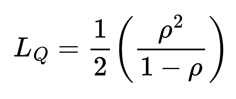
The equation above only applies for utilization factors less than 1. In this equation the average queue size is 0 if the utilization factor is 0, which makes sense as that corresponds to either 0 arrivals or an infinite service rate. However, we can see that the average queue size increases as the utilization factor approaches one. At the limit of the utilization factor reaching 1, the average queue size then goes towards infinity.

Results and Comparison with Theory

We’ve developed a simple simulation for an M/D/1 queue. Now, let’s run this simulation over 24 hours for different scenarios and compare some of the average queue size results with theory. In all of these scenarios the expected arrival rate will stay at a value of 10. Only the service rate will be varied to show different utilization factors.

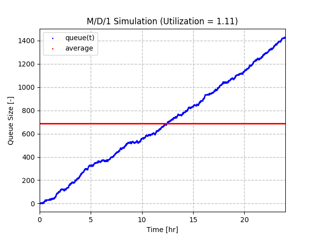
The first example is an arrival rate of 10 and a service rate of 9, which gives us a utilization factor of 1.11. You can see that the queue grows from 0 to just over 1400 items. Since there is a difference in 1 item per minute in the expected rates, this makes sense as there are 1440 minutes in a 24 hour period. There is also some noticeable noise and variation as the queue increases due to the natural variability in the arrival amounts. Also note that the average queue size was approximately 700, but this would continue to increase toward infinity if the simulation were allowed to continue past 24 hours.

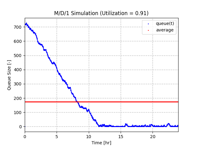
To test the opposite scenario, we can show a queue where the service rate is 11 and the arrival rate is 10, which gives a utilization factor of 0.91. The queue is also given the initial condition of starting with 720 items. You can see that the queue size drops on average at a rate of 1 item per minute. Afterwards it tends to bounce around 0 due to variation in the arrivals. The average queue size here is about 175, which is primarily due to the fact that the queue started at a large value.

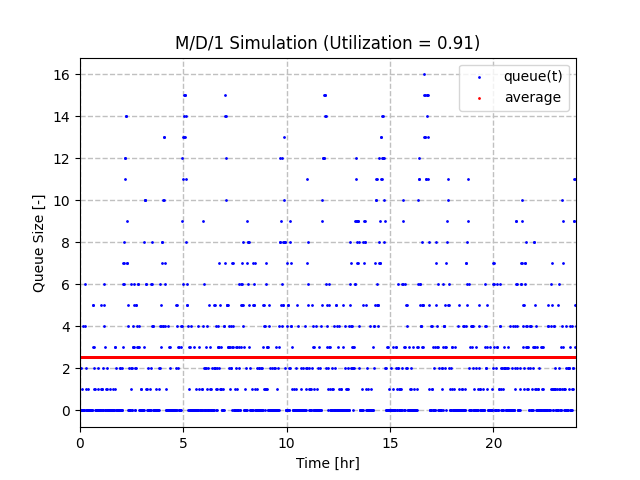
Let’s look at the same scenario as the last one, but starting at a queue size of 0. With a utilization factor of 0.91, we see a maximum queue size of 16. However, the average is much lower at 2.5. This is the right order of magnitude as the theoretical average queue size for an M/D/1 queue with a utilization factor of 0.91 is 4.6.

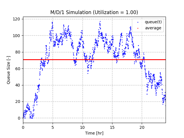
Finally, we can look at the result when the utilization factor is 1.0. Here the queue size increases to near 120 with an average size of approximately 70. Referencing the queue size equation for an M/D/1 queue, we would expect an average queue of this size to have a utilization factor of 0.993. So there are some slight differences between our simulation model and the closed form equation. That being said, this graph illustrates that a queuing system near 100% utilization has wide swings in queue size. This is because the expected values are balanced and it’s more or less up to luck if the queue will continue to increase or not. Either way, you can’t assume the queue won’t increase in this scenario.

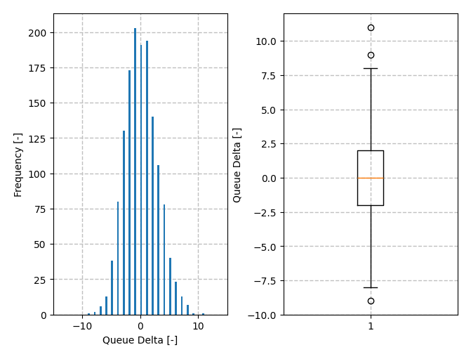
For the case of 100% utilization, it’s also interesting to look at the distribution of changes in queue size each minute throughout the 24 hour simulation. The histogram below shows that the deltas are mostly centered around zero. Note that there are some long tail deltas greater than 10 as it’s possible to get arrivals that are much larger than 10 (e.g. 60), but the minimum number of arrivals that can happen are 0. The whisker and box plot also shows some outliers to the high side. It’s not obvious from these charts, but the average delta is also slightly positive. This is partly because if the queue size is less than 10, then the server cannot use its full capacity. In other words, a queue can’t have a negative length.

Conclusions

I hope you’ve gotten something out of this small exploration into queueing theory from the perspective of a die roll. My goal was to provide a more intuitive example of what is meant by an arrival process following a Poisson distribution. Also, it’s useful to see a time-series representation of these queues since most of the equations are presented for average queue lengths for a system that has stabilized in some form. We saw that the simulation does agree qualitatively with theory in that average queue size tends to increase significantly as utilization approaches 100%. It’s also interesting to see that because queues cannot be negative, there’s almost a guarantee that the queue will have some average size simply due to variation in the arrivals and departures.