Can IOPS Be Estimated from fsync?
Introduction
Write speeds can be one of the main bottlenecks in databases. Doing something like write-back caching can help with spikes in traffic, but ultimately if there is high throughput, a single node will reach its limit. Many databases use the syscall fsync as a component of finishing a transaction to maintain durability. One of the side effects of ensuring data durability through the use of fsync is higher latency. And because this syscall can take up the lion’s share of the total latency for a database transaction, it’s safe to say that the rate at which fsync can be called will serve as a factor to how many transactions can be processed per second [1].
The focus of this post isn’t actually to get into the details of how databases use fsync, but to dig into what are the performance limits of this syscall on some commodity servers. To do that, we’re going to explore I/O write performance on some gp2 EBS volumes on AWS EC2. We’ll look into how quickly fsync operations can be run and if there is any evidence of parallelization or aggregation. The goal here is to answer the question: Can IOPS be estimated from fsync alone?
Commodity Disks in the Cloud
Amazon Web Services (AWS) provides Elastic Block Store (EBS) as an option for persistent storage within the cloud. These are paired with EC2 instances to create the base file system in which applications can interact. We’re going to look at gp2 volumes from EBS, which are standard general-purpose SSD disks. The write throughput of a gp2 volume is measured in terms of I/O operations per second or IOPS. All gp2 volumes start out with a minimum of 100 IOPS and can go up to a maximum of 16000 IOPS. In between the min and max, 3 IOPS are added to the baseline for every GB of provisioned disk space. The equation for calculated baseline IOPS is as follows:
Baseline IOPS = min(max(100, 3 * SIZE_IN_GB), 16000)
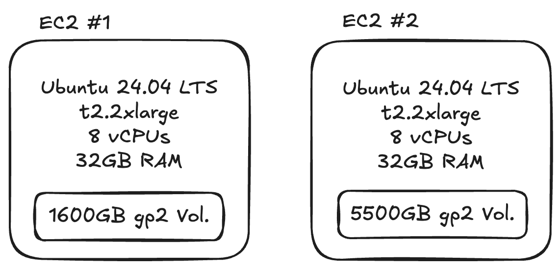
Note that gp2 volumes under 1000GB have the ability to burst temporarily up to 3000 IOPS [2]. To keep things simple, we’ll look at two different volume sizes: (1) 1600GB and (2) 5500GB, which will give us 4800 IOPS and 16000 IOPS, respectively. This allows us to explore the range of fsync latencies for different IOPS limits while also moving the baseline above 3000 IOPS to avoid the complexities of transient write capacity. These volumes were installed on t2.2xlarge EC2 instances (8 vCPUs / 32GB RAM) running Ubuntu 24.04 LTS (x86). A larger instance size was chosen to reduce the likelihood of bottlenecks beyond disk writes.
Latency with Fsync
It’s useful to consider the performance of a single fsync to give an idea of the disk speed. Percona used a python script in their article, which I have modified slightly to report the average fsync latency over 3000 samples [4].
# For original see: https://www.percona.com/blog/fsync-performance-storage-devices/

import os, sys, mmap
import time

# Number of fsync samples to take
N = 3000

# Open a file
fd = os.open("testfile", os.O_RDWR|os.O_CREAT|os.O_DIRECT )

m = mmap.mmap(-1, 512)
s = time.perf_counter()
for i in range (1, N):
   os.lseek(fd,os.SEEK_SET,0)
   m[1] = 1
   os.write(fd, m)
   os.fsync(fd)
e = time.perf_counter()
elapsed = e - s
dt_fsync = 1e6 * elapsed/N
iops = N / elapsed

print(f"Time elapsed for {N} fsyncs: {elapsed}")
print(f"Avg fsync dt: {dt_fsync} [usec]")
print(f"IOPS: {iops}")

# Close opened file
os.close( fd )
Running the script above on a 1600GB gp2 volume gave an average fsync latency of
4.25 ms, which corresponds to 235 IOPS. Recall from the equation in the previous section that a gp2 instance has 3 IOPS per GB of storage. Therefore an instance of 1600GB should be able to deliver up to 4800 IOPS. This means that it must be able to run multiple fsync operations together, perhaps through batching or parallelization, because running fsync serially will not get us up to that level of IOPS.
Benchmarking Latency and IOPS with FIO
To get more detailed results on the fsync latency and IOPS performance of gp2 volumes I’ve used fio (Flexible I/O Tester), which is an open source benchmarking tool that can generate a range of different I/O workloads. Starting off with a root volume size of 1600GB, the first test that was ran used this command structure to create random 4k writes:
fio \
    --name=random-write \
    --bs=4k \
    --end_fsync=1 \
    --fsync=1 \
    --iodepth=1 \
    --ioengine=posixaio \
    --numjobs=1 \
    --runtime=60 \
    --rw=randwrite \
    --size=100M \
    --time_based
This I/O workload simulates a worse-case scenario that could be encountered with a database installation as random writes tend to be slower than sequential ones. There is one job configured to run for 60s, writing 100MB repeatedly until the time is reached. It will also perform an fsync after every I/O operation as well as when the job ends. In this particular case, I set iodepth to 1, which means that only 1 unit of I/O will be kept in flight against the file. This is essentially the desired queue size from the application side. The results are shown below.
random-write: (g=0): rw=randwrite, bs=(R) 4096B-4096B, (W) 4096B-4096B, (T) 4096B-4096B, ioengine=posixaio, iodepth=1
fio-3.36
Starting 1 process
random-write: Laying out IO file (1 file / 100MiB)
Jobs: 1 (f=1): [w(1)][100.0%][w=996KiB/s][w=249 IOPS][eta 00m:00s]
random-write: (groupid=0, jobs=1): err= 0: pid=1949: Thu Mar  6 13:29:09 2025
  write: IOPS=256, BW=1024KiB/s (1049kB/s)(60.0MiB/60003msec); 0 zone resets
    slat (usec): min=2, max=927, avg= 8.00, stdev=11.55
    clat (nsec): min=1178, max=4494.4k, avg=94785.53, stdev=160874.28
     lat (usec): min=28, max=4502, avg=102.79, stdev=161.66
    clat percentiles (usec):
     |  1.00th=[   35],  5.00th=[   38], 10.00th=[   39], 20.00th=[   41],
     | 30.00th=[   43], 40.00th=[   44], 50.00th=[   46], 60.00th=[   48],
     | 70.00th=[   55], 80.00th=[   67], 90.00th=[  109], 95.00th=[  498],
     | 99.00th=[  766], 99.50th=[  930], 99.90th=[ 1237], 99.95th=[ 1401],
     | 99.99th=[ 2933]
   bw (  KiB/s): min=  968, max= 1112, per=100.00%, avg=1025.03, stdev=30.00, samples=119
   iops        : min=  242, max=  278, avg=256.25, stdev= 7.50, samples=119
  lat (usec)   : 2=0.01%, 4=0.01%, 50=65.26%, 100=24.40%, 250=1.68%
  lat (usec)   : 500=3.64%, 750=3.92%, 1000=0.74%
  lat (msec)   : 2=0.33%, 4=0.01%, 10=0.01%
  fsync/fdatasync/sync_file_range:
    sync (usec): min=2371, max=15410, avg=3788.90, stdev=652.71
    sync percentiles (usec):
     |  1.00th=[ 2868],  5.00th=[ 2999], 10.00th=[ 3064], 20.00th=[ 3261],
     | 30.00th=[ 3425], 40.00th=[ 3556], 50.00th=[ 3687], 60.00th=[ 3851],
     | 70.00th=[ 4015], 80.00th=[ 4228], 90.00th=[ 4555], 95.00th=[ 4883],
     | 99.00th=[ 5800], 99.50th=[ 6521], 99.90th=[ 8356], 99.95th=[ 8586],
     | 99.99th=[10290]
  cpu          : usr=0.56%, sys=0.77%, ctx=30737, majf=0, minf=27
  IO depths    : 1=200.0%, 2=0.0%, 4=0.0%, 8=0.0%, 16=0.0%, 32=0.0%, >=64=0.0%
     submit    : 0=0.0%, 4=100.0%, 8=0.0%, 16=0.0%, 32=0.0%, 64=0.0%, >=64=0.0%
     complete  : 0=0.0%, 4=100.0%, 8=0.0%, 16=0.0%, 32=0.0%, 64=0.0%, >=64=0.0%
     issued rwts: total=0,15362,0,15362 short=0,0,0,0 dropped=0,0,0,0
     latency   : target=0, window=0, percentile=100.00%, depth=1

Run status group 0 (all jobs):
  WRITE: bw=1024KiB/s (1049kB/s), 1024KiB/s-1024KiB/s (1049kB/s-1049kB/s), io=60.0MiB (62.9MB), run=60003-60003msec

Disk stats (read/write):
  xvda: ios=0/49108, sectors=0/1388608, merge=0/31216, ticks=0/55327, in_queue=55327, util=83.08%
There is a lot of detail in this output, but the parts we’re going to focus on are the averages
for lat (usec), iops, and sync (usec), which represent the application I/O latency, IOPS, and fsync latency, respectively [5]. We’ll make the simplifying assumption that the total latency is the sum of lat (usec) and sync (usec). One interesting observation is that the average fsync latency is measured as 3788.9 us (3.8 ms), which isn’t far from the 4.25 ms we measured using the python script earlier. The average IOPS were also comparable at 256. Next, let’s see what happened as iodepth was swept from 1 up to 80 for the 1600GB gp2 volume.
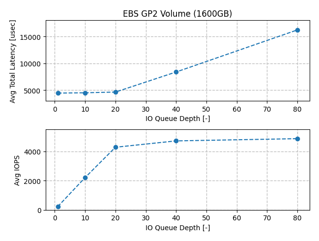
The first thing to observe is that the latency stayed relatively constant as iodepth went from 1 up to 20. We also got linearly increasing IOPS as a function of queue depth. The relationship is captured by Little’s Law, which states that the queue size (L) will equal the average arrival rate (λ) multiplied by the wait time an item spends in the system (W).

The average total latency was taken as the sum of the average lat (usec) and sync (usec) values. Note that IOPS linearly increased with iodepth between 1 and 20 because the latency was relatively constant in that range. For a 1600GB gp2 volume, we would expect a capacity
of 4800 IOPS, which is shown as a horizontal asymptote on the IOPS vs. Queue Depth chart.
Another interesting observation is that the total latency began to increase rapidly as
we reached the IOPS limit for a gp2 volume. This increase in latency offset the increase in iodepth such that no further increase in IOPS was achieved.
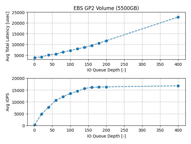
Next, let’s look at the results from the 5500GB gp2 volume. In this case iodepth was
increased from 1 up to 400. This size volume had a 16000 IOPS capacity, which we see via
the horizontal asymptote as iodepth was increased past 160. The total latency numbers increased from 3.89 ms up to 22.7 ms. Unlike the case with the 1600GB gp2 volume, latency steadily increased across the range of iodepth values, suggesting that at higher IOPS levels the system is unable to service each I/O unit immediately.
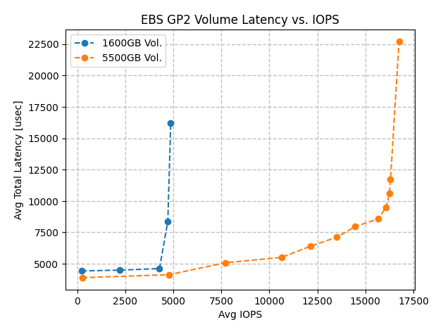
Finally, we can look at the 1600GB and 5500GB gp2 volume results together in terms of average total latency vs. IOPS. At roughly 4500 IOPS and below, each volume showed stable latency around 4 ms. The 1600GB volume quickly hit a wall at its 4800 IOPS limit and latency increased without any more write throughput. The 5500GB volume showed a latency curve that increases in slope as it got closer to the 16000 IOPS limit. This volume also had a wall, where IOPS could not move much further past 16000 without skyrocketing latency values.
Conclusions
When evaluating random write capabilities of a particular disk, the latency of a single fsync operation can provide some insight into its speed, however it’s not sufficient to know what the overall IOPS capacity is. We looked at test results from two sizes of AWS EBS gp2 volumes (1600GB and 5500GB) to better understand the IOPS vs. fsync latency relationship. These results showed that while the fsync latency for an I/O unit without a queue is around 4 ms, we could achieve up to 16000 IOPS on a 5500GB drive. This means that the system is capable of performing some sort of aggregation or parallelization of the fsync operations, which if only allowed to operate serially would limit us to approximately 250 IOPS. So if you have a disk where you’re unsure of its IOPS capacity, make sure to take the time to benchmark it. A back of the envelope calculation assuming the inverse of the fsync latency can be an order of magnitude off.